What Is a Deterministic Finite Automaton?

In the previous lesson, we explored alphabets, words, and languages. Today, we will see how these notions are used to define the deterministic finite automaton (DFA, for short).

One way to view automata is to look at them as computers with extremely limited memory. (We note that automaton refers to a single machine, and automata is the plural form). As the name suggests, deterministic finite automata are finite in the sense that an automaton has a finite number of internal states that it can be in at any given moment in its operation, and these states are the elements that serve as memory. This limitation is manifested in the fact that automata can remember information only by being in a specific state.

Before we describe automata formally, we start with an example that emphasizes how they work at their core, leading the way to a precise definition. It turns out that the automaton model lies at the heart of many interesting devices around us, including the digital safe box discussed below.

Example: How Does a Digital Safe Box Think?

You’ve probably seen one of these safe boxes in a hotel room.
We consider here one aspect of the digital safe box — setting up a password.
To set up a password, the user needs to open the door and press the reset button, enter a new password, and finally press the confirmation key $\#$.

The user must press the reset button first. Only after that he can enter numbers or press reset again to start over, until the confirmation key is pressed.

For simplicity, we consider a variant of a digital safe box that allows passwords consisting of two distinct numbers: an even number followed by an odd number. The available numbers are $1$, $2$, $3$, and $4$. Thus, in addition to the reset button and confirmation key, the safe box has four additional buttons corresponding to these numbers.

The interaction between the user and the safe box can be viewed as a finite sequence of actions where each action amounts to pressing a button. This suggests that we can view interactions as words by modeling each action as a letter.

Formally, consider the alphabet $\Sigma = \{ 1, 2, 3, 4, r, \#\}$, where each letter corresponds to pressing a button. For example, the letter $r$ corresponds to pressing the reset button, and the letter $3$ corresponds to pressing the $3$-button.

The word $w = r23\#$ describes an interaction where the user first presses the reset button, then enters the password $23$, and finally presses the confirmation key. The word $w$ is legal in the sense that it describes a successful setup of a password. Indeed, it starts and ends with $r$ and $\#$, respectively, and the password in between consists of two distinct numbers from the set $\{1, 2, 3, 4\}$ where the first is even and the second is odd.

Note that $r111r23\#$ is also a legal word because it starts with $r$, and after the last reset the user enters an allowed password followed by $\#$.

An example of a non-legal word would be a word that contains no $\#$ or more than one $\#$, a word that does not start with $r$, or a word where the password entered after the last reset contains repeating numbers, etc.

The digital safe box should be able to distinguish between legal and non-legal words, and it is no surprise that this logic can be carried out with a finite-state structure that keeps track of the needed information.

Let’s think about it. Assuming that we receive an input word $w$ once, one letter at a time, from left to right, we only need to remember a finite amount of information to decide whether $w$ is legal: (1) Does $w$ start and end with $r$ and $\#$, respectively?; (2) Does the password after the last reset consist of exactly two numbers — an even number followed by an odd number?; and (3) Does $\#$ appear exactly once in $w$?

To answer point (1), we only need to remember a finite amount of information: the first and last letters of the input word. Point (2), however, is less trivial, yet it requires us to remember the sequence of numbers entered so far after the last seen reset, and since an allowed password is of length 2, the total amount of information we need to remember here is finite as well. Finally, point (3) requires only finite information: we just need to remember if $\#$ has appeared yet.

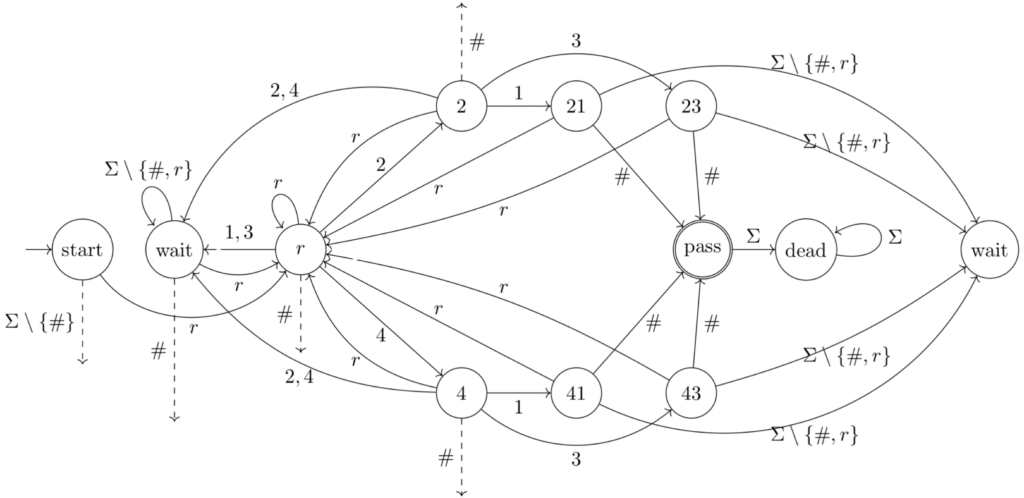
The following diagram represents a deterministic finite automaton implementation of the safe box:

Whew! Don’t worry — let’s unpack this step by step. The logic is straightforward, even if the diagram looks complex at first.

The above figure describes the automaton as a state diagram, which is a directed graph whose vertices correspond to states of the automaton (a vertex is labeled with the name of the corresponding state), and edges correspond to transitions of the automaton (an edge is labeled with a set of letters from the alphabet $\Sigma = \{ 1, 2, 3, 4, r, \#\}$; the destination of an edge specifies the state we should move to upon reading a letter labeled on that edge).

The automaton moves between its states depending on the current state and the input letter it receives at the moment, making its decision in a fully determined way.
For example, if the automaton is in the $r$-state and reads the input letter $2$, then it follows the $2$-labeled transition leading to the $2$-state. Moreover, if we are in the $\text{dead}$-state, then reading any letter from $\Sigma$ leads to the same $\text{dead}$-state.

For readability, we drew the $\text{wait}$-state twice, and dashed transitions lead to the $\text{dead}$-state.

Some of the states are drawn as double circles — these are accepting states — modeling successful interaction. The rest of the states are rejecting, modeling failed interaction. In our example, the $\text{pass}$-state is the only accepting state.

There is a single initial state having an unlabeled arrow entering it — this is where the run of the automaton starts, before receiving any input letter. Our initial state is denoted $\text{start}$.

We note that each state “remembers” some information. For example, if the automaton is in the $r$-state (remembering that the last read letter is $r$) and it receives the input letter $2$, then it moves to the $2$-state (remembering that we’ve read the password $2$ after the last reset). If the automaton, however, reads the input letter $1$ from the $r$-state, then it moves to the $\text{wait}$-state where it waits for the next reset. Note that this is the desired behavior since an allowed password does not start with $1$. Finally, reading $\#$ from the $\text{wait}$-state leads to the $\text{dead}$-state (remembering that the pattern of a legal word was violated).
Note that once we enter the $\text{dead}$-state, we can no longer reach the accepting $\text{pass}$-state.

Let’s consider running the automaton on a few input words to get a sense of how it works.
First, assume the automaton receives the following input word $w = r23\#$. Since $w$ is legal, we expect running the automaton on it to end up in the accepting $\text{pass}$-state. Indeed, when starting at the $\text{start}$-state and then read $w$, the automaton moves through the following sequence of states $s = \text{start}, r, 2, 23, \text{pass}$ following the labeled path $\text{start} \xrightarrow{r} r \xrightarrow{2} 2 \xrightarrow{3} 23 \xrightarrow{\#} pass$.

Next, if the automaton reads the legal input word $r111r23\#$, it also ends up in the accepting $\text{pass}$-state since it follows the sequence $s = \text{start}, r, \text{wait}, \text{wait}, \text{wait}, r, 2, 23, \text{pass}$. Here, the automaton moves to the $\text{wait}$-state after detecting a disallowed password and remains there until the next reset is seen.

However, if the automaton reads the non-legal input word $w = r21$, it ends up in the rejecting $\text{21}$-state since it follows the sequence $s = \text{start}, r, 2, 21$.

We denote such sequences of states as runs, which will be defined formally in the next section.

By carefully examining the structure of the automaton, it is not hard to verify that runs that end in the accepting $\text{pass}$-state are those that correspond to legal input words. Thus, the automaton successfully distinguishes between legal and non-legal words. Essentially, the only way to end up in the $\text{pass}$-state is by reading $\#$ from one of the states that remember an allowed password after the last reset ($21, 23, 41, 43$), as required.

Now that we’ve seen the safe box example, we can formalize the notions and define everything precisely.

Formal Definition of a Deterministic Finite Automaton

From this point, we study and develop the theory of automata abstractly without any particular application in mind.

We start with the formal definition of deterministic automata:

Definition — Syntax of a DFA

A deterministic finite automaton (DFA) $\mathcal{A}$ is a 5-tuple $\mathcal{A} = \langle \Sigma, Q, q_0, \delta, F\rangle$ where:

$\Sigma$ is an alphabet.
$Q$ is a finite set of states.
$q_0\in Q$ is the initial state.
$\delta: Q\times \Sigma \to Q$ is the transition function.
$F\subseteq Q$ is the set of accepting states.

Every DFA $\mathcal{A} = \langle \Sigma, Q, q_0, \delta, F\rangle$ has at least one state — the initial state $q_0$.

The transition function $\delta$ takes as input a pair $(q, \sigma)\in Q\times \Sigma$ of a state $q$ and a letter $\sigma$, and specifies that the automaton moves to the state $\delta(q, \sigma)$ when the letter $\sigma$ is read from the state $q$.

We proceed with notation that is useful for reasoning about automata, both now and in subsequent lessons.

For states $q, s\in Q$ and a letter $\sigma\in \Sigma$, we say that $\langle q, \sigma, s\rangle$ is a transition of $\mathcal{A}$ when $s = \delta(q, \sigma)$. We refer to $\sigma$ as the label of that transition, and refer to $s$ as the $\sigma$-successor of $q$. We sometimes write the transition $\langle q, \sigma, s\rangle$ as $q \xrightarrow{\sigma} s$.

Note that the transition function is deterministic in the sense that it specifies exactly one $\sigma$-successor for every state and letter $\sigma$.

Recall that $F$ is the set of accepting states. A state that is not accepting is rejecting. Thus, $Q\setminus F$ is the set of rejecting states.

The above definition describes the syntax of a deterministic automaton — given an object, we can easily verify whether it is a DFA by checking if it describes a 5-tuple satisfying the conditions above.

Example

Consider the DFA $\mathcal{A} = \langle \Sigma, Q, q_0, \delta, F\rangle$ where:

$\Sigma = \{ 0, 1\}$,
$Q = \{ q_0, q_1, q_2\}$,
$F = \{ q_1\}$,
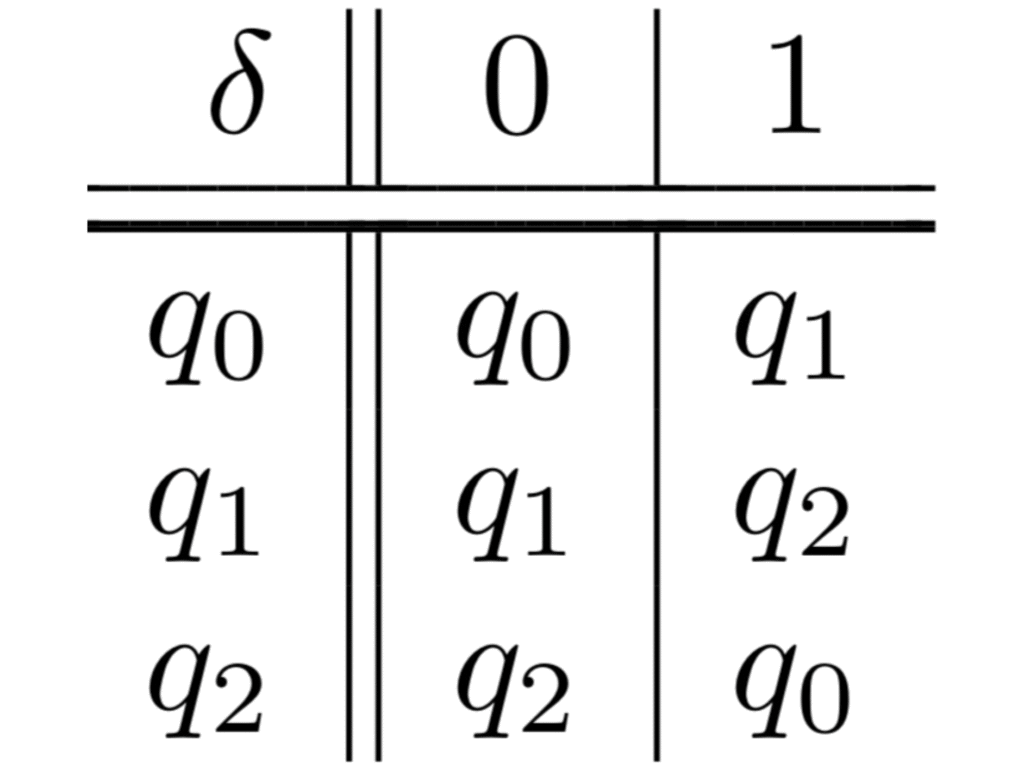
The transition function $\delta$ is described by the following table:

The following is the state-diagram of $\mathcal{A}$:

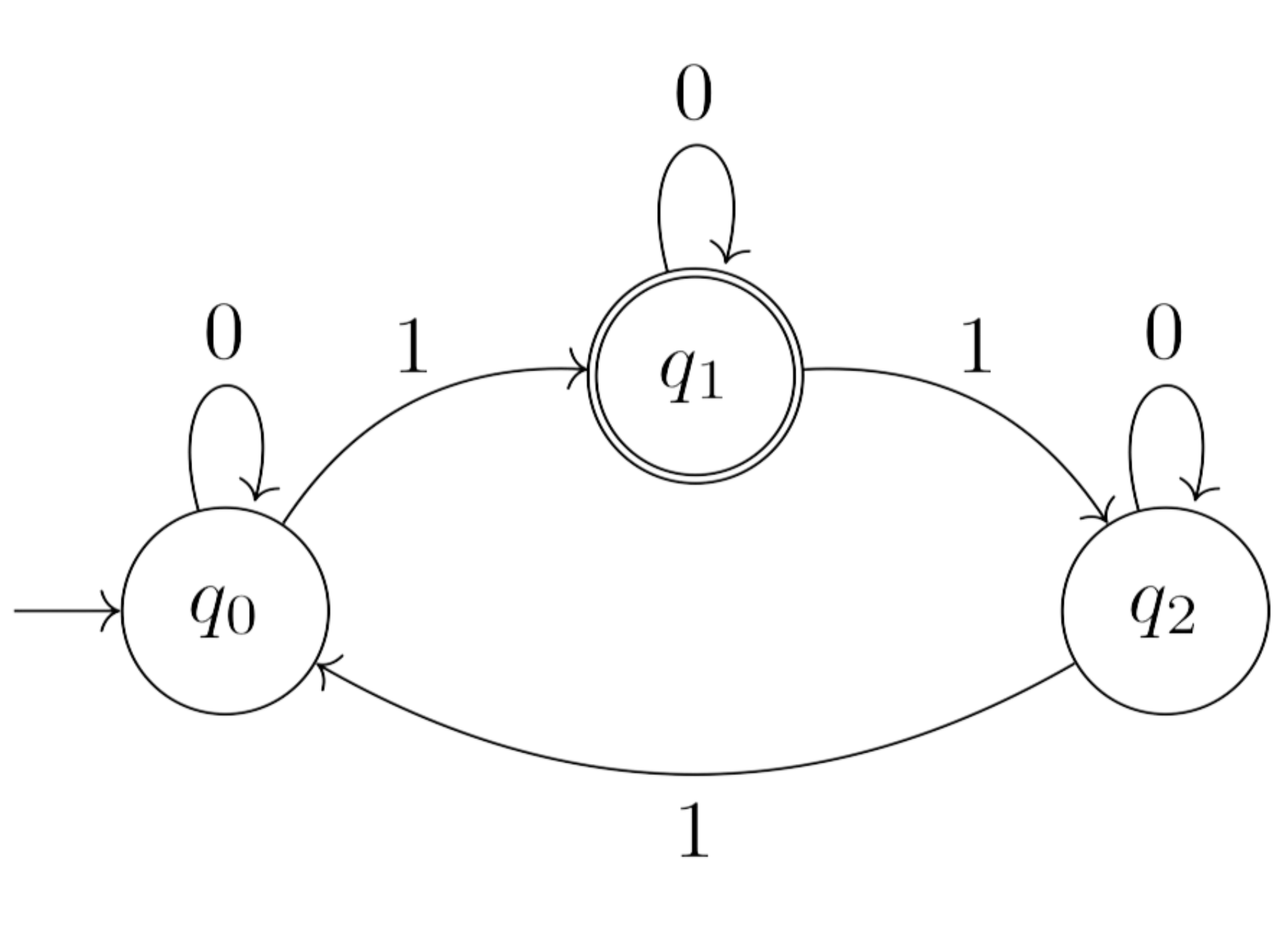
The initial state $q_0$ has an unlabeled arrow entering it.
The state $q_1$ is accepting — drawn as double circles.
The DFA $\mathcal{A}$ has 3 states: the initial state $q_0$, $q_1$ and $q_2$. The only accepting state is $q_1$, meaning that $q_0$ and $q_2$ are rejecting states.
The DFA $\mathcal{A}$ is defined over the binary alphabet $ \{ 0, 1\}$.
The transition function $\delta$ is deterministic as it specifies a single successor for every state and letter. For example, by reading the letter $0$ from the state $q_1$, we have exactly one destination to move to, which is the state $q_1$, and reading the letter $1$ from the state $q_2$ leads only to $q_0$.
$\langle q_0, 1, q_1\rangle$ is a transition, and $q_1$ is the $1$-successor of $q_0$.
$\langle q_0, 0, q_0\rangle$ is a self-loop labeled with $0$ (a $0$-labeled transition from a state to itself).

Next, we define the semantics of a DFA — the language it recognizes. For that, we first need a few more definitions. We start with runs.

Consider a DFA $\mathcal{A} = \langle \Sigma, Q, q_0, \delta, F \rangle$ and an input word $w = \sigma_1\cdot \sigma_2 \cdots \sigma_n\in \Sigma^*$, where $\sigma_i\in \Sigma$ for all $1\leq i \leq n$. A run of $\mathcal{A}$ on $w$ is a sequence of states $r = r_0, r_1, \ldots, r_n$ that satisfies the following:

The state $r_0$ is the initial state of $\mathcal{A}$ ($r_0 = q_0 $), and
For all $ 0 < i \leq n$, it holds that $r_i = \delta(r_{i-1}, \sigma_i)$.

Thus, $r$ starts at the initial state and follows the transition function of the automaton. Note that $r$ is unique as $r_i$ is the only $\sigma_i$-successor of $r_{i-1}$; in other words, a deterministic automaton has a single run on a given input word.

In the literature, such runs are also termed computations.

A run $r$ is accepting (rejecting) if it ends in an accepting (rejecting, respectively) state. Then, a DFA $\mathcal{A}$ accepts (rejects) an input word $w$ when the run of $\mathcal{A}$ on $w$ is accepting (rejecting, respectively).

We sometimes write a run $r = r_0, r_1, \ldots, r_n$ over $w = \sigma_1\cdot \sigma_2\cdots \sigma_n$ more explicitly as a sequence of successive transitions $r_0\xrightarrow{\sigma_1} r_1 \xrightarrow{\sigma_2} r_2 \cdots r_{n-1} \xrightarrow{\sigma_n} r_n$.

Intuitively, runs describe how a DFA processes a given input word, and the set of accepting states $F$ defines the acceptance criterion — whether a run ends in an accepting state determines whether the DFA accepts the corresponding input word. This leads to the following definition, relating automata with languages:

Definition — Semantics of a DFA

Consider a DFA $ \mathcal{A} = \langle \Sigma, Q, q_0, \delta, F\rangle$. The language of $\mathcal{A}$, denoted $L(\mathcal{A})$, is the set of words that $\mathcal{A}$ accepts. Thus, $L(\mathcal{A}) = \{ w\in \Sigma^*: \mathcal{A} \text{ accepts } w\}$.

Then, $\mathcal{A} $ recognizes a language $L\subseteq \Sigma^*$ when $L(\mathcal{A}) = L$.

Using this notion of a language recognized by a DFA, we can now define regular languages. This is the first nontrivial class of languages studied in the context of computation, and it captures exactly what can be described using finite automata.

Definition

Consider a language $L\subseteq \Sigma^*$. We say that $L$ is regular when there is a DFA that recognizes it.

We denote by $\text{REG}$ the class of regular languages.

Now that we have defined regular languages formally, we illustrate the concept with an explicit DFA example, showing the language it recognizes and the runs corresponding to specific input words.

Example

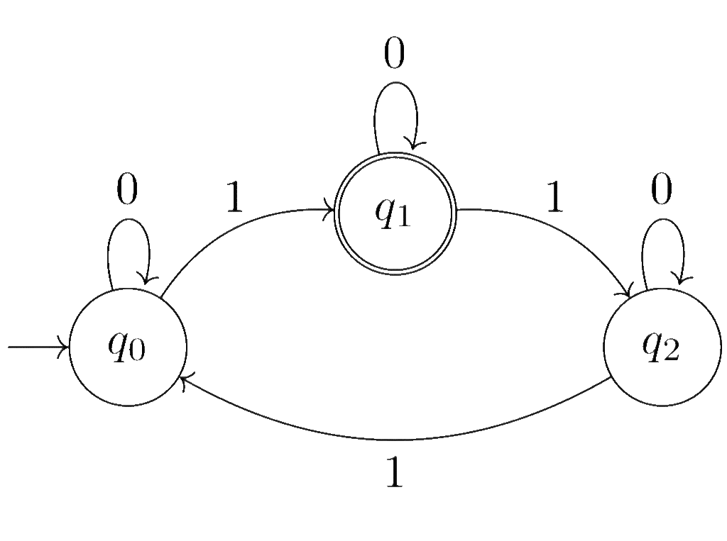
Recall the DFA $\mathcal{A} = \langle \{ 0, 1\}, \{q_0, q_1, q_2 \}, q_0, \delta, \{q_1\} \rangle$ from the previous example:

Consider the input words $u = 001011$ and $w = 0011011$.
The run $r_u$ of $\mathcal{A}$ on $u$ equals $r_u = q_0, q_0, q_0, q_1, q_1, q_2, q_0$, and the run $r_w$ of $\mathcal{A}$ on $w$ equals $r_w = q_0, q_0, q_0, q_1, q_2, q_2, q_0, q_1$.

Both runs can be written more explicitly as $$r_u = q_0 \xrightarrow{0} q_0 \xrightarrow{0} q_0 \xrightarrow{1} q_1 \xrightarrow{0} q_1 \xrightarrow{1} q_2 \xrightarrow{1} q_0$$ and $$r_w = q_0\xrightarrow{0} q_0 \xrightarrow{0} q_0 \xrightarrow{1} q_1 \xrightarrow{1} q_2 \xrightarrow{0} q_2 \xrightarrow{1} q_0 \xrightarrow{1} q_1 $$

The former run ends in the rejecting state $q_0$ and the latter run ends in the accepting state $q_1$; accordingly $u\notin L(\mathcal{A})$ but $w\in L(\mathcal{A})$.

For a word $x\in \{0, 1\}^*$, let $\#_1(x)$ denote the number of $1$’s appearing in $x$. For example, $\#_1(\epsilon) = 0$, $\#_1(u) = 3$ and $\#_1(w) = 4$. The automaton $\mathcal{A}$ recognizes the language $$L(\mathcal{A}) = \{ x\in \{ 0, 1\}^*: \#_1(x) \equiv 1 \mod 3 \}$$

Essentially, the state $q_i$ remembers that the number of $1$’s read so far has remainder $i$ when divided by $3$. Reading a $0$ does not change this remainder, so the automaton stays in the state $q_i$, while reading a $1$ moves it to the state $q_{(i + 1) \mod 3} $. This way, $\mathcal{A}$ keeps track of the remainder and accepts only when the run ends in $q_1$, specifying that the remainder corresponding to the read input equals 1.

The language $L = \{ x\in \{ 0, 1\}^*: \#_1(x) \equiv 1 \mod 3 \}$ is regular since $\mathcal{A}$ is an automaton that recognizes it. Thus, we can write $L\in \text{REG}$.

What’s Next

Today we covered deterministic finite automata — what they are and how they operate. In the next lesson, we will continue exploring DFAs, mainly working through several DFA examples and practice designing automata.

Stay tuned!

Automata and Regular Languages — Lessons